Rendering in Haskell, Part 7: Onward to Photon Mapping
So far in this series, I’ve been generating images using standard ray-tracing, a local illumination technique. Ray-tracing is easy to implement, relatively fast, but unfortunately doesn’t produce very realistic images. To make more realistic images, I need to switch to a global illumination system. I’ve chosen to use Photon Mapping.
It’s worth going back and thinking about the ray-tracing algorithm I have been using so far works, and why it doesn’t produce particularly good images.
Ray Tracing
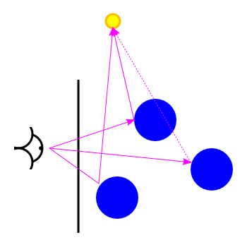
In ray-tracing, rays are traced starting from the camera, into the scene, and from the surfaces in the scene, directly to the lights. With the exception of rendering reflective surfaces, this technique puts an upper bound on the number of rays needed (number of pixels times number of lights). It is however, completely the opposite way around to how light actually works in the real world.
Real Life
In real life of course, light ‘rays’ start from the light sources, not the camera, and bounce around the scene until they either reach the camera (dashed line in diagram above), or vastly more likely, terminate in a surface, warming it ever so slightly. (Why vastly more likely? Think about the surface area of your eye’s pupils, compared to the surface area of everything else in the room). While it would be possible to simulate this process, it would be very inefficient in terms of producing an image: the vast majority of rays cast from the light sources wouldn’t contribute anything towards the final image.
Photon Mapping
Photon Mapping attempts to combine these two approaches (faster, rays traced from eye, low quality; slower, rays traced from light, high quality). To do this, it takes a two-pass approach.
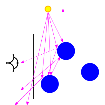
On the first pass, rays are traced from the light source, into the scene:
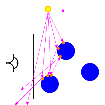
Each time a ray hits a surface, a record is kept of the ray, the position, and the light intensity and color. Light is allowed to bounce around the scene: for every surface interaction, there is a chance the ray will bounce off (adjusted for surface color), or if that chance fails, the ray is taken to have been absorbed.
(More reflective, light-colored surfaces have a higher chance of bouncing the ray; less reflective, dark-colored surfaces will have a lower chance of bouncing the ray).
So photon mapping is a probabilistic technique: it won’t generate the same image each time, and the more light rays are used, the better the final image will be.
Once enough rays have been bounced around the scene, the second pass comes into play. Rays are traced from the camera into the scene:
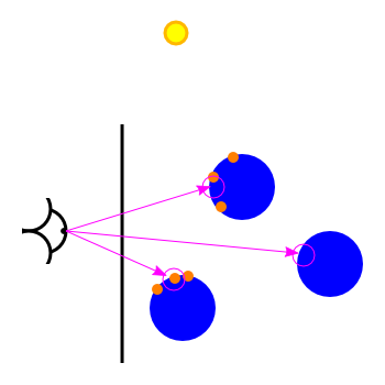
At each surface intersection, any nearby stored records of light are combined together to give an estimate of the diffuse light at that point.
(Obviously there is a tradeoff to be made here: if the area for considering nearby points is too small, the final image will appear ‘grainy’; and if the area is too small, the final image will be blurred, and there will be no sharp shadow features).
When tracing the rays from the camera, no further bounces are needed, except for the case of shiny reflective surfaces, or refractive volumes.
Published: Saturday, December 05, 2015
You may be interested in...
Hackification.io is a participant in the Amazon Services LLC Associates Program, an affiliate advertising program designed to provide a means for sites to earn advertising fees by advertising and linking to amazon.com. I may earn a small commission for my endorsement, recommendation, testimonial, and/or link to any products or services from this website.